Content
- Node embeddings (lecture 3.1)
- Random walk for node embeddings (lecture 3.2)
- Embed entire graph (lecture 3.3)
1. Node embedding
Instead of traditional feature engineering, vector embedding of nodes can be beneficial in
- measure the similarity between nodes
- encode network information
- potential use for many downstream predictions
encode-decoder
Definitions:
- V is the vertex set
- A is the adjacency matrix
- graph $G : { V, A }$
- encoder: map nodes to embeddings, $ENC(v) = z_v$
- similarity function $f$, e.g., $f(u,v) \approx z_v^T z_u$
- decoder: decode embeddings to the similarity score
2. Random walk
Random walk: given a graph and a starting point, select a neighbor of it at random and move to the selected neighbor, and repeat it again and again.
Random walk embeddings: 1) estimate the probability of visiting node v on a random walk starting from node u using some random walk strategy R, 2) optimize embeddings to encode these random walk statistics.
random walk optimization: $Loss = \sum_{u \in V} \sum_{v \in N_R(u)} - log(P(v|z_u))$, where $P(v|z_u) = \frac{exp(z_u^T z_v)}{\sum_{n \in V} exp(z_u^T z_n)}$, use softmax because we want node v to be most similar to node u out of all nodes n.
negative sampling: to reduce computational complexity, only sample a subset of all the nodes: \(log(P(v|z_u)) = log(\frac{exp(z_u^T z_v)}{\sum_{n \in V} exp(z_u^T z_n)}) \approx log(\sigma(z_u^T z_v)) - \sum_{i=1}^k log(\sigma(z_u^T z_{n_i}))\), where $n_i \in P_V$, $P_V$ is random distribution other than uniform distribution.
node2vec
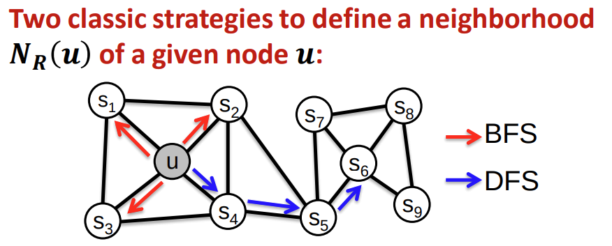
two strategies to define a neighborhood: global: depth first search; local: breadth first search.
3. Embed entire graph
simple approach
sum of the embeddings
virtual node
sub-graph as a virtual node
hierarchical embeddings


